Back in 1972, almost half a century ago, David Lorge Parnas published an iconic paper entitled “On the Criteria to Be Used in Decomposing Systems into Modules” 1. In it he discusses modularization as a mechanism for improving the flexibility and comprehensibility of a system while allowing the shortening of its development time, and also presents a criterion for effectively carrying out the decomposition of a system into modules.
When I first read this paper I was impressed by how relevant and practical it is. I stumbled on it while reading through an online discussion on the topic of object oriented programming. Yet again someone had published a post criticizing the fundamental concepts of OOP and in the discussion there was a comment pointing out to the author that he had misinterpreted the concept of encapsulation in his critique, linking to the paper.
It was in this paper that the concept of information hiding, closely related to encapsulation, was first described. This concept plays a central role in the strategy for effective system modularization, as I’ll describe in the following sections.
Benefits of an effective modularization
Modularization is the division of a system or product into smaller, independent units that work alongside each other for implementing said system or product requirements. In regard to software projects, it is applied to a system at its higher levels of abstraction (ex: microservices architecture) and at its lower levels as well (ex: object oriented class design).
When performed effectively, modularization brings many benefits, among them:
- Managerial: Development time should be shortened because separate teams would work on each module with little need for communication
- Flexibility: It should be possible to make drastic changes to one module without a need to change others
- Comprehensibility: It should be possible to study the system one module at a time, and the whole system can therefore be better designed because it is better understood
A strong indicator that a system has not been properly modularized is not reaping the benefits listed above. The challenge is then to define, and follow, a criterion that leads the system towards an effective modularized structure.
According to D.L. Parnas, one might choose between two distinct criteria for breaking a system into modules:
- The Procedural Criterion: Make each major step in the processing a module, typically begining with a rough flowchart and moving from there to a detailed implementation
- The Information Hiding Criterion: Every module is characterized by its knowledge of a design decision which it hides from all others
In the next section we will use an example system to demonstrate how following the second criterion leads the system towards a much more effective modularized structure than following the first one, and why the first criterion should actually never be followed alone unless there’s a strong motivation to do so.
Example system: Scheduling Calendar
Consider a Scheduling Calendar system that implements the following features:
- As an organizer, I want to create a scheduled event so that I can invite guests to attend it
- As an organizer, I want to be informed of conflicting guests schedules so that I’m able to propose a valid event date
- As a participant, I want automatic reminders to notify me of upcoming events I should attend so that I don’t miss them
Let’s exercise both criteria for sketching this system’s modularized structure. Notice that I will not be using class diagrams as not to induce an OOP bias in this exercise.
Using the procedural criterion
A straightforward procedure for implementing the event creation feature is:
- Read JSON input with the proposed event information (Date, Title, Location, Participants)
- Validate against a
user_schedulesdatabase table that all participants can attend to this new event - In case one or more participants isn’t able to attend, throw an exception informing it, otherwise proceed
- Insert an entry in an
eventstable and one entry for each participant in auser_schedulestable
We also need to define a procedure for implementing the automatic notification feature:
- Setup a notifier task that continuously polls the
user_schedulestable - Select all
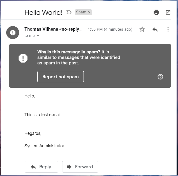
user_scheduleswhosenotification_datecolumn is due andnotifiedcolumn isfalse - For each resulting entry, send an e-mail reminder message to the corresponding event participant
- Then, for each resulting entry, set the
notifiedcolumn value withtrue
The database schema is being loosely defined since it’s not the central point here to discuss it. It’s sufficient to say that, considering a relational database and the third normal form, three tables would suffice the storage necessities of this exercise: events, users and user_schedules.
Based on these two procedures, we might define the following modules for the Scheduling Calendar:
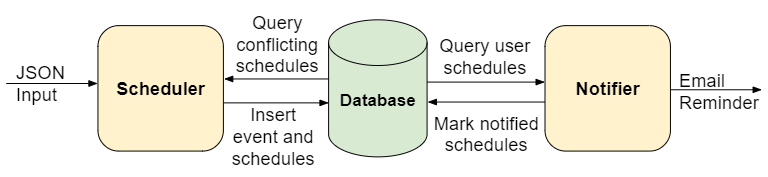
Naturally, following this criterion leads to modules with several responsibilities. The scheduler module is parsing the input, validating data, querying the database and inserting new entries. The notifier module is also querying the database, modifying entries, preparing and sending e-mail messages.
Using Information Hiding as a criterion
Information hiding is the principle of segregation of the design decisions in a system that are most likely to change, thus protecting other parts of the system from extensive modification if a design decision is indeed changed. The protection involves providing a stable interface which isolates the remainder of the system from the implementation.
To apply this principle we start with the system requirements and extrapolate them, anticipating all possible improvement/change requests we can think of that our users, or any stakeholder actually, might ask:
- Handle different input formats (ex: JSON, XML)
- Allow the addition and removal of participants after the creation of an event
- Allow users to customize the frequency of event reminders (ex: single vs multiple notifications per event)
- Implement different notification types (E-mail, SMS, Push Notification)
- Support a different storage medium (ex: SQL Database, NoSQL Database, In Memory - for testing purposes)
Hopefully most of them will make sense, but it’s always a good idea to involve a colleague to validate them before making a design decision that might be expensive to change later on.
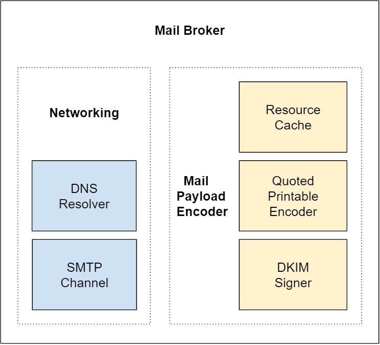
Now the challenge is to define a system structure that isolates these possible changes to individual modules. Here’s a proposition:
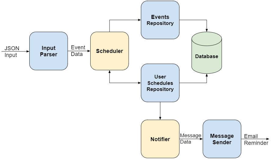
As you can see, several specialized modules appeared (in blue), segregating system responsibilities.
The InputParser module hides the knowledge of what input format is being used, converting the JSON data into an internal representation. If we are required to support XML instead, it’s just a matter of implementing another kind of InputParser and plug it into our system.
The Repository modules hide the knowledge of the storage medium from the Scheduler and Notifier modules. Again, if we are required to change persistence to another kind of database we can do so without ever touching Scheduler and Notifier modules. On top of that the specialized repository modules can assimilate data modification and querying responsibilities, making it easier to implement functional changes to events and user schedules.
A MessageSender module is employed for hiding the knowledge of how to send specific notification types. It receives a standardized message request from the Notifier module and sends the corresponding e-mail reminder. If we need to start sending SMS reminders we just have to implement a new kind of MessageSender and plug it to the output of the Notifier.
With the extraction of these specialized modules the original Scheduler and Notifier modules become thinner and take on a new role acting as higher level services, orchestrating lower level modules for implementing system operations. D.L. Parnas reasoned about this hierarchical structure that is formed while decomposing the system, pointing out that it favors code reuse, leveraging productivity. He also warned against lower level modules making use of higher level modules, as it would break the hierarchical structure.
Conclusion
In this exercise I tried to demonstrate how using the information hiding criterion naturally leads to an improved system structure when compared to using the procedural criterion. The latter results in less modules that aggregate many responsibilities, while the former promotes the segregation of responsibilities into several specialized modules. These specialized modules become the foundation of a hierarchical system structure that not only improves comprehension of the system but also it’s flexibility.
The proposed strategy for effective system modularization is then to:
- Enlist all operations the system is required to implement
- Anticipate possible improvement/change requests for these operations
- Identify design decisions likely to change, prioritizing them if necessary
- Extract specialized modules that encapsulate these design decisions
- Establish and maintain a clear hierarchical structure within the system
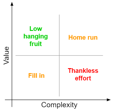
The first two steps will help visualize what the system design decisions are, upon which the information hiding criterion (third and fourth steps) is applied. Depending on the scale of enlisted design decisions susceptible to change a prioritization step may come in handy for directing development efforts and maximizing value:
In closing I would like to add another quote from D.L. Parnas own conclusion pertaining this strategy’s third step, in which specialized modules are extracted from the system:
Each module is then designed to hide such a decision from the others. Since, in most cases, design decisions transcend time of execution, modules will not correspond to steps in the processing. To achieve an efficient implementation we must abandon the assumption that a module is one or more subroutines, and instead allow subroutines and programs to be assembled collections of code from various modules.
For me this quote captures the main paradigm shift from procedural to object oriented programming.
Sources
[1] Parnas, D.L. (December 1972). “On the Criteria To Be Used in Decomposing Systems into Modules” (PDF)