Graph databases are much more efficient than traditional relational databases for traversing interconnected data. The way they store data and execute queries is heavily optimized for this use case, and one property in particular is key for achieving such higher performance: index-free adjacency.
This short article first analyzes the complexity of data traversal in relational databases, then explains how graph databases take advantage of index-free adjacency for traversing data more efficiently.
Relational Databases
Consider a social application in which users can follow each other, and its simplified database schema presented below:
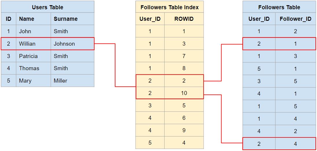
In this illustrative schema a Users table stores application users profiles, and a Followers table stores unidirectional “follower” relationships between users. An Index is also used to speed-up queries against the Followers table (represented in yellow).
Suppose we want to know whether or not it’s possible to reach an specific “Target User” starting from “Source User” with at most “N” steps, how do we implement this in SQL?
Since SQL is designed as a declarative programming language for querying data contained in a relational database we need help of an imperative programming language for implementing this traversal algorithm, and fortunately most database systems do support structured programming out of the box for writing functions and stored procedures.
Regardless of the specific database and programming language used, the traversal code should look similar to the code example provided below:
bool CanReachTarget(int[] sourceIds, int targetId, HashSet<int> visitedIds, int steps)
{
    if (steps == 0)
        return false;

    int[] followersIds = ExecuteQuery<int[]>(
        "SELECT Follower_ID FROM Followers WHERE User_ID in ({0});",
        sourceIds
    );

    if (followersIds.Contains(targetId))
    {
        return true;
    }
    else
    {
        visitedIds.AddRange(sourceIds);
        sourceIds = followersIds.Except(visitedIds).ToArray();
        return CanReachTarget(sourceIds, targetId, visitedIds, steps - 1);
    }
}
At each level of the recursion the function will fetch all followers IDs at that level, check whether or not the target ID is present, return true in case it’s present or go one level deeper in case it’s not, keeping track of aready visited elements. If the function runs out of steps during the recursion it will return false, since it failed to reach the target ID.
Let’s exercise this algorithm with data from figure 1, starting from “Willian Johnson” (ID = 2) and trying to reach “Mary Miller” (ID = 5) with at most 3 steps:
| sourceIds | targetId | visitedIds | steps | followersIds | contains? | |
|---|---|---|---|---|---|---|
| #1 | [2] | 5 | [ ] | 3 | [1, 4] | false |
| #2 | [1, 4] | 5 | [2] | 2 | [1, 2, 3, 4, 5] | true |
Notice that “Mary Miller” was found at the second level, and the function will return true in this case.
Now, let’s analyze the time complexity of this algorithm. You may have already realized that it’s performing a Breadth First Search (BFS), offloading most of the work to the database query engine. The BFS part executes O(V + E) operations, where V is the number of users whose followers are fetched from the database and E the aggregated number of followers from this group of users. The cost to fetch followers for each user considering a B-Tree index is O(log(n)), where n is the length of the followers table. Hence, the resulting time complexity will be O(V * log(n) + E).
Without the index things would be much worse, since a full table scan would be necessary to fetch followers, yielding O(V * n + E) time complexity in the worst case.
Graph Databases
As I’ve said at the beginning of this article graph databases take advantage of index-free adjacency for traversing data more efficiently. Figure 2 presents a logical representation of how data from figure 1 would be organized in a graph database:
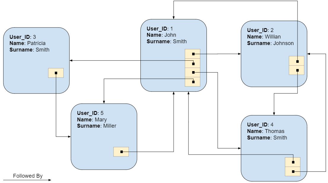
Instead of relying on a global index for accessing connected nodes, each node directly references its adjacent nodes. Even though the lack of a global index for nodes relationships is what gives the index-free adjacency property its name, you can think that each node actually holds a mini-index to all nearby nodes, making traversal operations extremely cheap.
As to leverage this structure, graph databases perform traversal queries natively, being able to execute the BFS algorithm from the previous section entirely whithin the database query engine. The BFS part will still execute O(V + E) operations, however the cost to fetch a user node followers will go down to O(1), running in constant time, since all followers are directly referenced at the node level.
You may be thinking:
What about accessing the query starting node in the first place, wouldn’t that require a global index?
And you’re completely right, in order to get to the starting point of the traversal efficiently we will have to rely on an index lookup. Again, considering a B-Tree index, this will run in O(log(n)) time in addition to the traversal.
The resulting time complexity for the query will be simply O(V + E + log(n)), much better than for relational databases, specially when the number of users (n) gets larger.
A lot of factors that affect database performance were left out of the analysis for simplicity, such as file system caching, data storage sparsity, memory requirements, schema and query optimizations.
There’s no single universal database that performs greatly in all scenarios. Different kinds of problems may be better solved using different kinds of databases, if you can afford the additional operational burden. As with most decisions in software development, a reasonable approach is to lay down your requirements and analyze whether or not tools available to you meet them before jumping to a new ship.