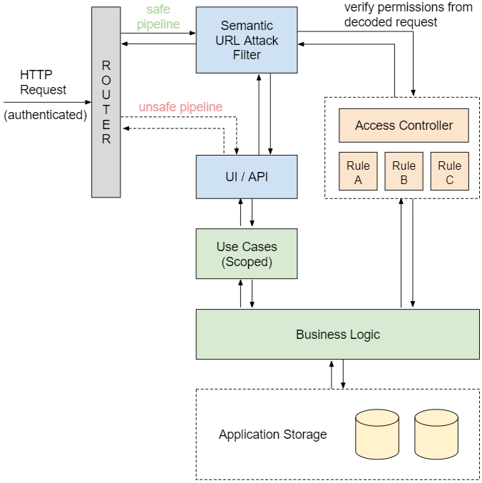
In my previous post I have briefly described my recent adventures in the DeFi space and how I’ve built an experimental decentralized options exchange on ethereum with solidity programming. If you haven’t read it yet, feel free to follow the link below for more context:
In this post I’m gonna talk about liquidity pools. More specifically about a linear interpolation based liquidity pool I have developed for my experimental options exchange, whose source code and brief documentation you can find in the project’s GitHub repository:
First we will recall what’s a liquidity pool and the purpose it serves (feel free to jump ahead if you’re already familiary with it). Then I’ll present my linear interpolation liquidity pool proposal and explain how it works, it’s advantages and disadvantages.
What’s a liquidity pool?
A liquidity pool is a smart contract that gathers funds from individuals denominated liquidity providers which are then used to facilitate decentralized trading. As the name suggests liquidity pools provide “liquidity” to the market, i.e., they make it possible for traders to quickly purchase or sell an asset without causing a drastic change in the asset’s price, and without subjecting traders to unfair prices, which would be one of the consequences of lack of liquidity.
DeFi liquidity pools emerged as an innovative and automated solution for addressing the liquidity challenge on decentralized exchanges. They replace the traditional order book model used in traditional exchanges (such as the NYSE) which is not applicable to most cryptocurrencies platforms mainly due to their highly mutable nature, i.e., in a matter of a couple of hundreds of milliseconds an entire order book can change as a result of orders being created, updated, fulfilled and cancelled, which would be extremely costly in a platform like ethereum on account of transaction fees.
One could say that achieving efficient pricing is among the biggest challenges for implementing a successful liquidity pool. Typically the price of an asset varies according to supply and demand pressures. If there’s too much supply prices will drop, since sellers will compete against each other for offering the most competitive price. Likewise if demand is up to the roof prices will rise, since buyers will fight amongst themselves to offer the best price for purchasing an asset.
Several models have been proposed and are being used in DeFi to address this challenge. Uniswap liquidity pools famously use the constant product formula to automatically adjust cryptocurrencies exchange prices upon each processed transaction. In this case market participants are resposible for driving exchange rates up/down by taking advantage of short-lived arbitrage opportunities that appear when prices distantiate from their ideal values.
Nonetheless a supply/demand based pricing model, such as Uniswap’s, is in my opinion unfit for pricing options, since an option price is not entirely the result of supply and demand pressures, but rather directly dependent on its underlying’s price. This observation motivated me to propose a linear interpolation based liquidity pool model, as we’ll see in the next section.
The linear interpolation liquidity pool
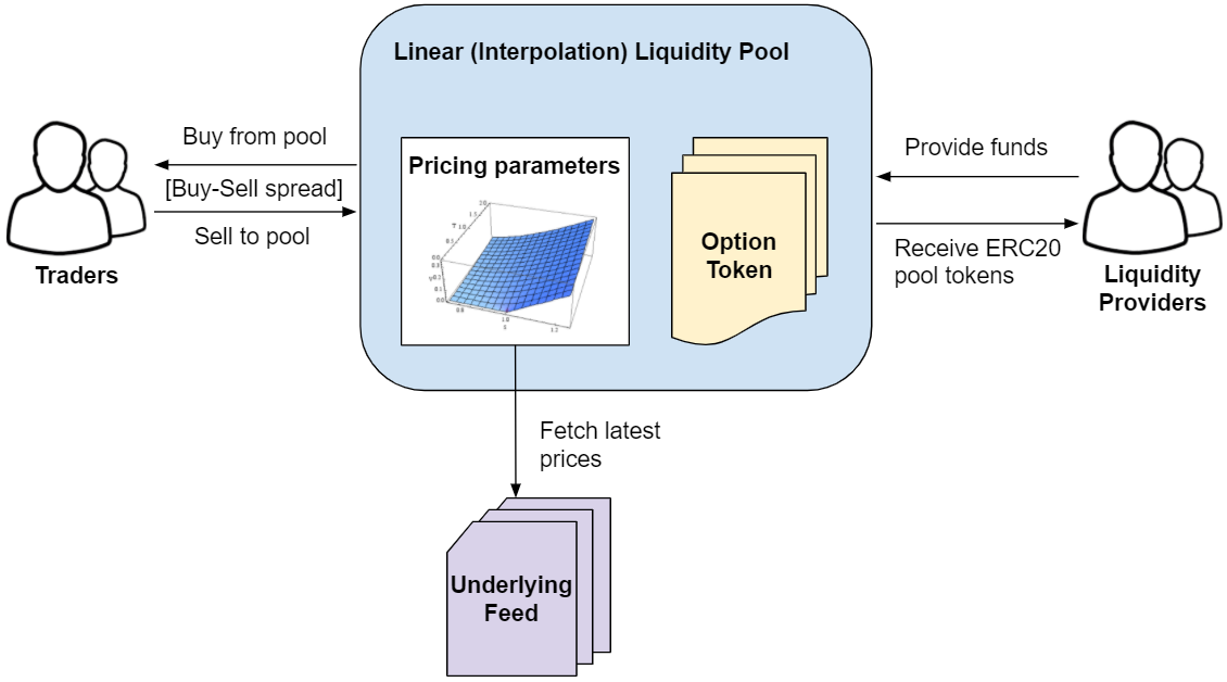
The diagram below illustrates how the linear interpolation liquidity pool fits in the options exchange trading environment, how market agents interact with it, and provides some context on the pool pricing model:
Market Agents
On one side of the table we have options traders that interact with the pool by either buying options from it or selling options to it. The pool first calculates the target price for an option based on its internal pricing parameters (more on that latter) and then applies a fixed spread on top of it for deriving the buy price above the target price, and sell price below the target price. This spread can be freely defined by the pool operator and should be high enough for ensuring the pool is profitable, but not too high as to demotivate traders.
Below are the solidity function signatures available for traders to interact with the pool:
function queryBuy(string calldata symbol) external view returns (uint price, uint volume);

function querySell(string calldata symbol) external view returns (uint price, uint volume);

function buy(string calldata symbol, uint price, uint volume, address token)
    external
    returns (address addr);

function sell(string calldata symbol, uint price, uint volume) external;
- The
queryBuy function receives an option symbol and returns the spread-adjusted “buy” price and available volume for traders to buy from the pool
- Similarly the
querySell function receives an option symbol and returns the spread-adjusted “sell” price and available volume the pool is able to purchase from traders
- Traders can then call the
buy function to purchase option tokens specifying the option symbol, queried “buy” price, desired volume and the address of the stablecoin used as payment
- Or call the
sell function to receive payment for option tokens being sold to the pool specifying the option symbol, queried “sell” price and the pre-approved option token transfer volume
On the other side of the table we have liquidity providers. They interact with the pool by depositing funds into it which are used to both i) allocate collateral for writing new option tokens for selling to traders and ii) allocate a reserve of capital for buying option tokens from traders.
Below is the solidity function signature liquidity providers should call for providing funds to the pool:
function depositTokens(address to, address token, uint value) external;
Liquidity providers receive pool tokens in return for depositing compatible stablecoin tokens into the pool following a “post-money” valuation strategy, i.e., proportionally to their contribution to the total amount of capital allocated in the pool including the expected value of open option positions. This allows new liquidity providers to enter the pool at any time without harm to pre-existent providers.
Funds are locked in the pool until it reaches the pre-defined liquidation date, whereupon the pool ceases operations and profits are distributed to liquidity providers proportionally to their participation in the total supply of pool tokens.
Even so, since the pool is tokenized, liquidity providers are free to trade their pool tokens in the open market in case they need to recover their funds earlier.
Pricing Model
The pool holds a pricing parameters data structure for each tradable option, as shown below, which contains a discretized pricing curve calculated off-chain based on a traditional option pricing model (ex: Monte Carlo) that’s “uploaded” to the pool storage. The pool pricing function receives the underlying price (fetched from the underlying price feed) and the current timestamp as inputs, then it interpolates the discrete curve to obtain the desired option’s target price. That’s it, just simple math.
struct PricingParameters {
    address udlFeed;
    uint strike;
    uint maturity;
    OptionsExchange.OptionType optType;
    uint t0;
    uint t1;
    uint[] x;
    uint[] y;
    uint buyStock;
    uint sellStock;
}
Notice the t0 and t1 parameters, which define, respectively, the starting and ending timestamps for the interpolation. Also notice the x vector, which contains the underlying price points, and the y vector, which contains the pre-computed option price points for both the starting timestamp t0 and the ending timestamp t1 (see example snippet below). These four variables define the two-dimensional surface that the pool contract uses to calculate option prices.
 // underlying price points (US$)
x = [1350, 1400, 1450, 1500, 1550, 1600, 1650];

y = [
     // option price points for "t0" (US$)
    27, 42, 62, 87, 118, 152, 191,

    // option price points for "t1" (US$)
    22, 36, 56, 81, 111, 146, 185
];
This example snippet defines price points for a hypothetical ETH call option with strike price of US$ 1.500 and an interpolation period starting at 7 days to maturity and ending at 6 days to maturity, resulting in the pricing surface plotted below:
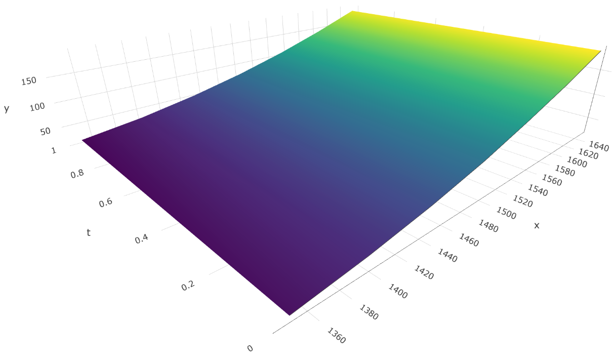
By following this approach the more heavy math is performed off-chain, since it would be unfeasible/too damn expensive to run a Monte Carlo simulation or any other option pricing method on ethereum, and actually a waste of capital, as interpolating a preprocessed discretized curve achieves similar end results with much less on-chain computational effort.
Advantages
Below I provide a couple of reasons of why I believe this approach will appeal to both options traders and liquidity providers:
- Changes to the underlying price are instantly reflected on the option price, meaning that the pool won’t be subject to arbitrage that would otherwise reduce its gains and that traders can rest assured they are getting fair, transparent prices when interacting with the pool.
- Zero slippage, since options prices aren’t dependent on offer/demand pressures, making it simpler to trade larger option token volumes.
- Lightweight pricing model, allowing a single pool to trade multiple symbols, which can potentially reduce the pool returns volatility due to the effects of diversification.
Disadvantages
I also see some operational/structural disadvantages of this design:
- Necessity to update pricing parameters on a regular basis, possibly daily, to prevent pool prices from being calculated using an outdated pricing curve that would result in pricing inefficiencies.
- Dependence on underlying price feed oracles. While the option price itself isn’t subject to direct manipulation one could try manipulating the underlying price feed instead, hence the importance of adopting trustworthy oracles.
- Requirement of an operator for overseeing pool operations such as registering tradable options, updating pricing parameters and defining buy-sell spreads.
Closing thoughts
This linear interpolation liquidity pool design adds up to the decentralized options exchange environment presented in my previous blog post. It’s been implemented as a decoupled, independent component with the goals of pricing efficiency, operational flexibility and design extensibility in mind.
I believe that, once deployed, this pool will be attractive for both traders, which will have access to more efficient prices with zero slippage, and liquidity providers, which will experience less volatility in their returns considering that a diversified options offer is added to the pool.
Next steps for this project include: backtesting of the liquidity pool to further validate its model and to estimate the appropriate parameters for launching; optimizations to solidity code for reducing gas consumption; and the development of the dapp front-end to make the exchange accessible to non-developers. Stay tuned!