Graph theory is extensively studied, experimented on and applied to communications networks 📡. Depending on a communication network’s requirements it may benefit from adopting one or another network topology: Point to point, Ring, Star, Tree, Mesh, and so forth.
In this post I analyze a network topology based on unweighted random regular graphs, and evaluate its robustness for data replication amid partial network disruption. First I present the definition of this kind of graph and describe its properties. Then I implement and validate a random regular graph generation algorithm from the literature. Finally I simulate data replication for varying degrees of partial network disruption and assess this topology effectiveness.
Supporting source code for this article can be found in this GitHub repository.
Definition
A regular graph is a graph where each vertex has the same number of neighbors; i.e. every vertex has the same degree or valency. The image below shows a few examples:
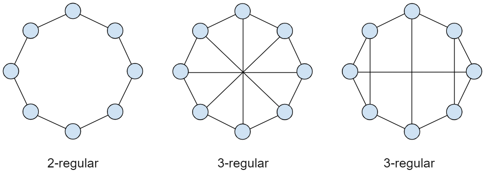
These sample graphs are regular since we can confirm that every vertex has exactly the same number of edges. The first one is 2-regular (two edges per vertex) and the following two are 3-regular (three edges per vertex).
Even though 0-regular (disconnected), 1-regular (two vertices connected by single edge) and 2-regular (circular) graphs take only one form each, r-regular graphs of the third degree and upwards take multiple distinct forms by combining their vertices in a variety of different ways.
More broadly we can denote Gn,r as the probability space of all r-regular graphs on n vertices, where 3 ≤ r < n. Then, we define a random r-regular graph as the result of randomly sampling Gn,r.
Properties of random regular graphs
There are at least two main properties that are worth exploring in this article. It is possible to prove that as the size of the graph grows the following holds asymptotically almost surely:
- A random r-regular graph is almost surely r-connected; thus, maximally connected
- A random r-regular graph has diameter at most d, where d has an upper bound of Θ(logr−1(nlogn)) [1]
The connectivity of a graph is an important measure of its resilience as a network. Qualitatively we can think of it as how tolerant the topology is to vertices failures. In this case, the graph being maximally connected means it’s as fault tolerant as it can be in regard to its degree.
Also relevant for communication networks is the graph diameter, which is the greatest distance between any pair of vertices, and hence is qualitatively related to the complexity of messaging routing within the network. In this case, the graph diameter grows slowly (somewhat logarithmically) as the graph size gets larger.
Graph generation algorithm
A widely known algorithm for generating random regular graphs is the pairing model, which was first given by Bollobas2. It’s a simple algorithm to implement and works fast enough for small degrees, but it becomes slow when the degree is large, because with high probability we will get a multigraph with loops and multiple edges, so we have to abandon this multigraph and start the algorithm again3.
The pairing model algorithm is as follows:
- Start with a set of n vertices.
- Create a new set of n*k points, distributing them across n buckets, such that each bucket contains k points.
- Take each point and pair it randomly with another one, until (n*k)/2 pairs are obtained (a perfect matching).
- Collapse the points, so that each bucket (and thus the points it contains) maps onto a single vertex of the original graph. Retain all edges between points as the edges of the corresponding vertices.
- Verify if the resulting graph is simple, i.e., make sure that none of the vertices have loops (self-connections) or multiple edges (more than one connection to the same vertex). If the graph is not simple, restart.
You can find my implementation of this algorithm in the following source file: RandomRegularGraphBuilder.cs.
Now that the algorithm is implemented, let’s evaluate that the properties described earlier truly hold.
Evaluating graph connectivity
In order to calculate a graph’s connectivity we need to ask for the minimum number of elements (vertices or edges) that need to be removed to separate the remaining vertices into isolated subgraphs.
We start from the observation that by selecting one vertex at will and then pairing it with all other remaining vertices in the graph, one at a time, to calculate their edge connectivity (i.e., the minimum number of cuts that partitions these vertices into two disjoint subsets) we are guaranteed to eventually stumble across the graphs own edge connectivity:
public int GetConnectivity()
{
    var min = -1;
    for (int i = 1; i < Vertices.Length; i++)
    {
        var c = GetConnectivity(Vertices[0], Vertices[i]);
        if (min < 0 || c < min)
            min = c;
    }
    return min;
}
The code above was taken from my Graph class and does just that from the array of vertices that compose the graph. The algorithm used in this code sample for calculating the edge connectivity between two vertices is straightforward, but a bit more extensive. Here’s what it does on a higher level:
- Initialize a counter at zero.
- Search for the shortest path between source vertex and destination vertex (using Depth First Search).
- If a valid path is found increment the counter, remove all path edges from the graph and go back to step 2.
- Otherwise finish. The counter will hold this pair of vertices’ edge connectivity.
It’s important to emphasize that this algorithm is intended for symmetric directed graphs, where all edges are bidirected (that is, for every arrow that belongs to the graph, the corresponding inversed arrow also belongs to it).
Once we are able to calculate a graph’s connectivity, it’s easy to define a unit-test for verifying that random regular graphs are indeed maximally connected:
[TestMethod]
public void RRG_Connectivity_Test()
{
    var n = (int)1e3;
    Assert.AreEqual(3, BuildRRG(n, r: 3).GetConnectivity());
    Assert.AreEqual(4, BuildRRG(n, r: 4).GetConnectivity());
    Assert.AreEqual(5, BuildRRG(n, r: 5).GetConnectivity());
    Assert.AreEqual(6, BuildRRG(n, r: 6).GetConnectivity());
    Assert.AreEqual(7, BuildRRG(n, r: 7).GetConnectivity());
    Assert.AreEqual(8, BuildRRG(n, r: 8).GetConnectivity());
}
This unit test is defined in the RandomRegularGraphBuilderTests.cs source file and, as theorized, it passes ✓
Evaluating graph diameter
The algorithm for calculating the diameter is much easier, particularly in the case of unweighted graphs. It boils down to calculating the maximum shortest path length from all vertices, and then taking the maximum value among them:
public int GetDiameter()
{
    return Vertices.Max(
        v => v.GetMaxShortestPathLength(Vertices.Length)
    );
}
This maximum shortest path length method receives an expectedVerticesCount integer parameter, which is the total number of vertices in the graph. This way the method is able to compare the number of vertices traversed while searching for the maximum shortest path with the graph’s size, and in case they differ, return a special value indicating that certain vertices are unreachable from the source vertex.
So after implementing this method I ran it against random regular graphs of varying sizes and degrees. The results are plotted below:
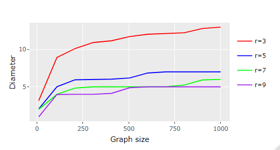
We can clearly confirm that the graph’s diameter flattens somewhat logarithmically as we increase the graph’s size and degree.
Since we are dealing with random graphs, instead of simply calculating the diameter for a single sample I generated one hundred samples per size and degree, and took their average. It’s worth noting that the inferred diameter standard deviation started reasonably small (less than 0.5) and diminished to insignificant values as the graph size and degree increased.
Data replication
In this study I simulated the propagation of information across random regular graphs accounting for disruption percentages starting from 0% (no disruption) up to 50% of the graph’s vertices. The simulation runs in steps, and at each iteration active vertices propagate their newly produced/received data to their neighbors.
At the beginning of each simulation vertices are randomly selected and marked as inactive up to the desired disruption percentage. Inactive vertices are able to receive data, but they don’t propagate it. The simulation runs until 100% of vertices successfully receive data originated from a source vertex chosen arbitrarily, or until the number of iterations becomes greater than the number of vertices, indicating that the level of disruption has effectively separated the graph into two isolated subgraphs.
Here’s the method that I implemented for running it for any given graph size and degree:
private static void SimulateReplications(int n, int r)
{
    Console.WriteLine($"Disruption\tIterations");

    for (double perc = 0; perc < 0.5; perc += 0.05)
    {
        var reached = -1;
        int iterations = 1;
        int disabled = (int)(perc * n);

        for (; iterations < n; iterations++)
        {
            var graph = new RandomRegularGraphBuilder().Build(n, r);

            var sourceVertex = 50; // Any
            var item = Guid.NewGuid().GetHashCode();
            graph.Vertices[sourceVertex].AddItem(item);

            graph.DisableRandomVertices(disabled, sourceVertex);
            graph.Propagate(iterations);

            reached = graph.Vertices.Count(n => n.Items.Contains(item));
            if (reached == n || iterations > n)
                break;
        }

        Console.WriteLine($"{perc.ToString("0.00")}\t{iterations}");
    }
}
The results for running it with parameters n = 1000 and r = [4, 8, 12] are given in the chart that follows:
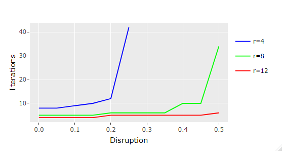
We can verify that the larger the graph’s degree, the less significant the effects of disruption levels are, which makes sense since intuitively there are much more path options available for the information to replicate.
In the simulation ran with parameters [n=1000, r=12] it was only required two additional iterations (6 in total) at 50% disruption for the source data to reach all graph vertices when compared with the base case in which all vertices were active.
For the lowest graph degree tested with [n=1000, r=4], however, the effects of disruption were quite noticeable, spiking to a total of 42 iterations for 25% disruption and not being able to reach the entirety of vertices for disruption levels above that (that’s why it’s not even plotted in the chart).
After some consideration, I realized that the spike in the number of iterations required for reaching all graph’s vertices in the simulation seems to occur when the chances of accidentally cutting the graph into two isolated subgraphs (while deactivating vertices) increase considerably. This probability can be roughly estimated as (1 - (1 - disruptionr)n), i.e., the probability of deactivating all neighbors of at least one graph vertex.
The following contour plot displays these probability estimates for graphs of size n=1000 for given disruption levels and graph degrees:
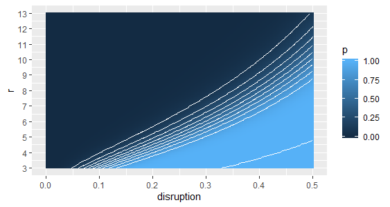
Now by analyzing the simulation iteration spikes on top of these probabilities we find that they started occurring when p neared 0.9. It’s important to highlight that as the probability of cutting off graph vertices increases, the number of simulation iterations required for reaching the totality of graph vertices becomes more volatile since, the way my code was devised, a new random regular graph is sampled and the current disruption level is randomly applied at each retrial. Nonetheless, as p nears 1.0, we are certain to end up with at least one disconnected vertex, meaning that we won’t be able to assess a valid number of simulation iterations for the replication to reach the entire graph.
Conclusion
This analysis has shown that from a theoretical point of view random regular graph topologies are particularly well suitable for data replication in applications where communication agents are faulty or cannot be fully trusted to relay messages, such as sensor networks, or reaching consensus in multi-agent systems.
As a result of being maximally connected, with proper scaling high levels of network disruption can be tolerated without significantly affecting the propagation of data among healthy network agents.
Lastly, the topology’s compact diameter favors fast and effective communication even for networks comprised of a large number of participating agents.
Sources
[1] B. Bollobás & W. Fernandez de la Vega, The diameter of random regular graphs, Combinatorica 2, 125–134 (1982).
[2] B. Bollobás, A probabilistic proof of an asymptotic formula for the number of labelled regular graphs, Preprint Series, Matematisk Institut, Aarhus Universitet (1979).
[3] Pu Gao, Models of generating random regular graphs and their short cycle distribution, University of Waterloo (2006).