In computational complexity theory problems are classified into classes according to the algorithmic complexity for solving them. Confusion often arises due to the fact that naming of these classes are not intuitive, and even misleading. For instance, many consider that the complexity class “NP” stands for “non-polynomial time” when it actually stands for “non-deterministic polynomial time”. Another common misconception is that problems that are elements of the “NP-hard” class are also elements of “NP”, which is not necessarily true.
The following table summarizes the most important complexity classes and their properties according to the current understanding in the field:
| P | NP | NP-complete | NP-hard | |
|---|---|---|---|---|
| Solvable in polynomial time | ✓ | |||
| Solution verifiable in polynomial time | ✓ | ✓ | ✓ | |
| Reduces any NP problem in polynomial time | ✓ | ✓ |
Each column lays down the pre-requisites a problem ought to fulfil for being considered a member of that complexity class. Notice that, trivially, all elements of “P” are also elements of “NP”, however the inverse cannot be alleged (at least while the P versus NP problem remains a major unsolved problem in computer science).
The next sections provide more details on these properties.
Solvable in polynomial time
Defines decision problems that can be solved by a deterministic Turing machine (DTM) using a polynomial amount of computation time, i.e., its running time is upper bounded by a polynomial expression in the size of the input for the algorithm. Using Big-O notation this time complexity is defined as O(n ^ k), where n is the size of the input and k a constant coefficient.
To put it briefly, a DTM executes algorithms the same way our modern computers do. It follows a set of pre-defined instructions (program), executing one instruction at a time, changing state and resolving the next instruction. We can imagine that at any given point in time there will be a history of executed operations and a set of predictable operations to follow based solely on the machine’s current state:
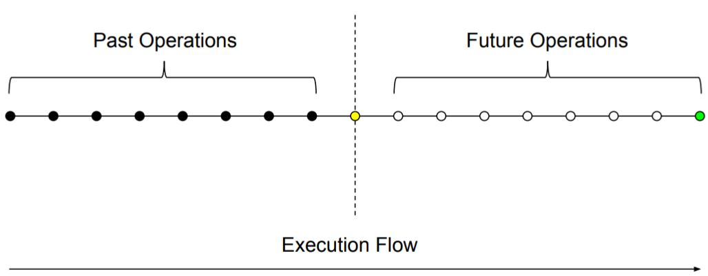
As long as there’s no external stimulus (randomness) involved, systems of this kind are deterministic, always producing the same output from a given initial state.
Solution verifiable in polynomial time
Defines decision problems for which a given solution can be verified by a DTM using a polynomial amount of computation time, even though obtaining the correct solution may require higher amounts of time.
There’s a straightforward brute force search approach for solving this kind of problems:
- Generate a solution Si from the space of every feasible solution (in constant time)
- Verify the correctness of the solution Si (in polynomial time)
- If solution Si correctly solves the problem, end execution
- Otherwise move to the next unvisited position i and repeat
It’s easy to see that this algorithm has time complexity O(k ^ n) * O(w), where w is the size of every feasible solution, since it iterates over the solution space and, for each possible solution, performs a verification that takes polynomial time. Typically solution spaces are not polynomial in size, yielding exponential (O(k ^ n)) or factorial (O(n!)) time complexity for this naive approach.
Here we introduce the non-deterministic Turing machine (NTM), a theoretical computer that can take this naive algorithm and run it in a polynomial amount of time:
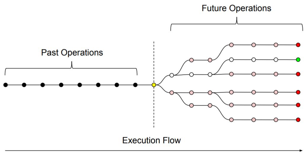
As figure 2 exemplifies, the NTM, by design, can be thought as capable of resolving multiple instructions simultaneously, branching into several execution flows, each one of them verifying a different solution to the decision problem, until one of them finds the correct one, halting the NTM.
NTMs only exist in theory, and it’s easy to understand why: Their capability for branching indefinitely into simultaneous execution flows would require an indefinitely large amount of physical resources.
Reduces any NP problem in polynomial time
Defines decision problems whose algorithms for solving them can be used to solve any NP problem after a polynomial time translation step. For instance, if we have a solver for a NP-hard problem, we can then build a solver for a NP problem as follows:
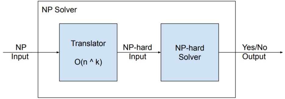
Hence, we are effectively reducing the NP-problem into the NP-hard problem for solving it. Intuitively problems that allow this are at least as hard as the hardest NP problem, otherwise they couldn’t be used to solve any NP problem.
As a consequence, if we were to find a polynomial time algorithm for solving a NP-hard problem (which is unlikely), then we could use it to solve any NP problem in polynomial time as well, implying that P = NP and solving the P versus NP problem.
Demonstration
For this demonstration we will use two well-known NP-complete problems:
- Knapsack problem: Given a set of items, each with a weight and a value, determine the number of each item to include in a collection so that the total weight is less than or equal to a given limit and the total value is as large as possible.
- Partition problem: Given a multiset S of positive integers, determine if it can be partitioned into two subsets S1 and S2 such that the sum of the numbers in S1 equals the sum of the numbers in S2.
First, consider the following solver for the knapsack problem in its decision form:
public class KnapsackProblemSolver
{
    public bool Solve(Item[] items, int capacity, int value)
    {
      /* ... */
    }
}
This solver will answer whether or not it’s possible to achieve a value combining the available items without exceeding the knapsack weight capacity, returning true in case it’s possible, false otherwise.
The Item data structure is presented below:
public class Item
{
    public int Value { get; set; }

    public int Weight { get; set; }

    public int Limit { get; set; }
}
Now, we want to implement a solver for the partition problem that answers whether or not a given multiset can be partitioned:
public class PartitionProblemSolver
{
    public bool Solve(int[] multiset)
    {
      /* ... */
    }
}
In order to do that we evaluate both problems objectives, translate the partition problem input accordingly, and feed it into the knapsack problem solver:
public class PartitionProblemSolver
{
    public bool Solve(int[] multiset)
    {
        var sum = multiset.Sum(n => n);
        if (sum % 2 == 1) // Odd sum base case for integer multiset
          return false;

        /* translate partition input into knapsack input */
        var items = multiset.Select(n => new Item { Value = n,  Weight = n, Limit = 1 }).ToArray();
        var capacity = sum / 2;
        var value = capacity;

        /* feed translated input into knapsack solver */
        return new KnapsackProblemSolver().Solve(items, capacity, value);
    }
}
Let’s analyze the translation step:
- It creates a set of items with a single item for each multiset element, assigning the item’s value and weight from the element’s own value.
- It defines the knapsack capacity as the expected sum for each partition. Hence, we know that if the capacity is completely filled, the combined weight of items inside and outside of the knapsack will be same.
- It defines the knapsack target value also as the expected sum for each partition. Since the defined capacity prevents a value higher than this from being achieved, the solver will return true if, and only if, the exact expected sum for each partition can be achieved, thus solving the partition problem.
If you found that fun, I suggest you try to reduce another NP problem to the knapsack problem. You’ll find out that each problem needs a slightly different approach, sometimes recurring to heuristics to make it work.
In the demonstration at the end of the article you may have noticed that I didn’t provide an actual implementation for solving the knapsack problem, however you can find one at the linked Wikipedia page, or in one of my GitHub repositories: https://github.com/TCGV/Knapsack
This is my take on the topic of complexity classes of problems, which I find of major importance for becoming a more effective, skillful software developer, giving us the tools for better analyzing and solving technical challenges. I hope you enjoyed it!